LightGCN: Evaluated and Enhanced

February 25, 2024

The work was accepted for the New in Machine Learning Workshop at the Thirty-seventh Conference on Neural Information Processing Systems (NeurIPS), 2023. Paper links: arXiv | Papers With Code | GitHub

This project builds on top of the paper LightGCN: Simplifying and Powering Graph Convolution Network for Recommendation by Xiangnan He, Kuan Deng, Xiang Wang, Yan Li, Yongdong Zhang, Meng Wang. The paper was published at SIGIR 2020.

Recommender Systems

Recommender Systems play a significant part in filtering and efficiently prioritizing relevant information to alleviate the information overload problem and maximize user engagement.

A recommender system makes a customized list of suggestions for users by looking at how they interact with others and their likes or dislikes of certain items. This process, known as Collaborative Filtering (CF), leverages the principle of user-item interactions to predict user preferences and make recommendations. In its basic form, collaborative filtering predicts the user-item interaction matrix as the dot product of user latent factors, denoted by $U$ and item latent factors, denoted by $V$, as follows:

\[\begin{equation} \mathbf{R} \approx \mathbf{UV}^\top \end{equation}\]

where $R$ is the predicted interaction matrix.

Graph Convolutional Networks

Graph Neural Networks (GNNs) and Graph Convolutional Networks (GCNs) utilize the concept of message passing to update node representations based on information from their neighbouring nodes. In this process, each node receives messages from its neighbours and aggregates these messages to obtain an updated embedding. This message passing can be formulated as follows:

\[\begin{equation} \mathbf{h}_v^{(k+1)} = \sigma \left(\sum_{u \in N(v)} \frac{1}{c_{u,v}} \mathbf{W}^{(k)}\mathbf{h}_u^{(k)}\right) \end{equation}\]

where \(\mathbf{h}_v^{(k)}\) represents the embedding of node $v$ at layer $k$, $N(v)$ denotes the set of neighboring nodes of $v$, $c_{u,v}$ is a normalization factor, \(\textbf{W}^{(k)}\) is a weight matrix at layer $k$, and $\sigma$ is an activation function.

LightGCN

LightGCN is a type of graph convolutional neural network (GCN), including only the most essential component in GCN (neighborhood aggregation) for collaborative filtering. Specifically, LightGCN learns user and item embeddings by linearly propagating them on the user-item interaction graph (bipartite graph), and uses the weighted sum of the embeddings learned at all layers as the final embedding.

The resulting aggregation function used in the graph convolutions of LightGCN is the following:

\[\begin{align} &\mathbf{e}_u^{(k + 1)} = \sum_{i \in N_u} \frac{1}{\sqrt{|N_u|}\sqrt{|N_i|}} \mathbf{e}_i^{(k)} &\mathbf{e}_i^{(k + 1)} = \sum_{u \in N_i} \frac{1}{\sqrt{|N_i|}\sqrt{|N_u|}} \mathbf{e}_u^{(k)} \end{align}\]

where $e_u^{(k)}$ and $e_i^{(k)}$ are embedding of user $u$ at layer $k$ and the the embedding of item $i$ at layer $k$ respectively. Therefore, each LightGCN layer computes new embeddings for each user and item by aggregating the embeddings of its immediate neighbours from the previous layer. With this design in place, the only trainable parameters are the embeddings at layers 0, more precisely the embeddings fed as input to the network. The final user or item embeddings obtained by a single forward pass of LightGCN are computed by taking the weighted sum of the embeddings at all layers, so the output embeddings of LightGCN are expressed as:

\[\begin{align} &\mathbf{e}_u = \sum_{k=0}^K \alpha_k \mathbf{e}_u^{(k)} &\mathbf{e}_i = \sum_{k=0}^K \alpha_k \mathbf{e}_i^{(k)} \end{align}\]

where $\alpha_k$ represents the weight associated with the embeddings computed by the $k$-th layer. The authors set all of the $\alpha_k$ values to $\frac{1}{K + 1}$.

In order to generate recommendations for a user, the authors take the inner product of its user embedding with the embeddings of all the other items and pick the items with the lowest inner product. The final predictions of LightGCN can be written as:

\[\begin{equation} \hat{y}_{ui}=\mathbf{e}_u^\top \mathbf{e}_i \end{equation}\]

Training LightGCN

To train the LightGCN model, we need an objective function that aligns with our goal for recommendation. We use the Bayesian Personalized Ranking (BPR) loss, which encourages observed user-item predictions to have increasingly higher values than unobserved ones, along with $L_2$ regularization:

\[\begin{equation} L_{BPR} = -\sum_{u=1}^{M}\sum_{i \in N_{u}}\sum_{j \notin N_{u}} ln \: \sigma (\hat{y}_{ui} - \hat{y}_{uj}) + \lambda ||\mathbf{E}^{(0)}||^{2} \end{equation}\]

where $\lambda$ is a hyperparameter that controls the $L_2$ regularization factor and $E^{(0)}$ is the embedding matrix at layer 0. The items that are not in the neighbourhood of a user are sampled uniformly.

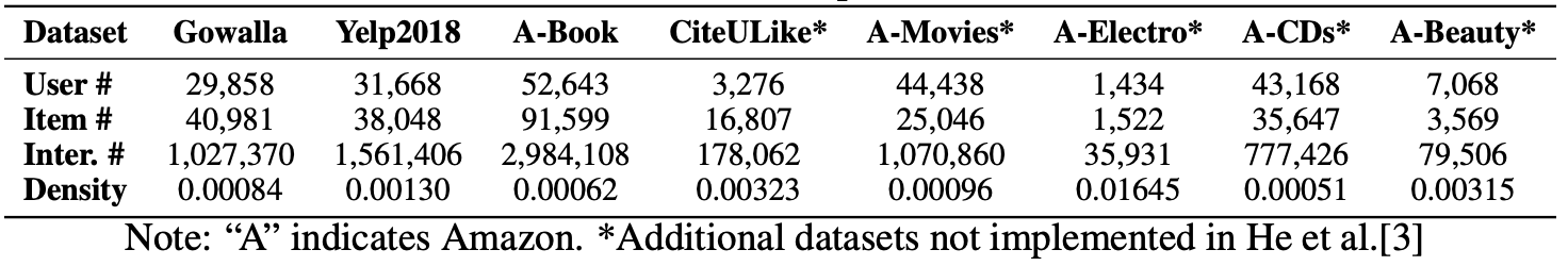
Datasets

In the original LightGCN paper, He et al. use the datasets Gowalla, Yelp2018, and Amazon-Book. To see how LightGCN performs in different domains and dataset sizes, we use five additional datasets: CiteULike, Amazon-Movies, Amazon-Electornics and Amazon-Beauty and Amazon-CDs. The statistics of the datasets are shown in the table below.

Evaluating LightGCN

We assess NDCG, recall, precision, diversity and fairness. We calculate diversity by the ILD. Users who make repeat purchases receive better recommendations than those exploring new items or with few interactions. To calculate fairness, we bin users by the number of interacted items. Similar recommendation performance across bins implies more fairness.

Our Enhancement: Approximate Personalised Propagation of Neural Predictions

Approximate Personalised Propagation of Neural Predictions (APPNP) is a GCN variant and an instance of graph diffusion convolution inspired by Personalised Page Rank (PPR). It derives from topic-sensitive PageRank approximated with power iteration propagating the final embeddings:

\[\begin{aligned} \textbf{Z}^{(0)} &= \textbf{E}^{(K)} \\ \textbf{Z}^{(k+1)} &= \alpha \textbf{Z}^{(0)} + (1 - \alpha)\hat{\tilde{\textbf{A}}}\textbf{Z}^{(k)} \\ \textbf{Z}^{(K)} &= \text{s} \left( \alpha \textbf{Z}^{(0)} + (1 - \alpha)\hat{\tilde{\textbf{A}}}\textbf{Z}^{(K-1)} \right) \end{aligned}\]

The final embedding matrix $\textbf{E}^{(K)}$ serves as the starting vector and teleport set with $K$ denoting power iteration steps. This method maintains graph sparsity without needing extra training parameters and prevents oversmoothing due to its teleport design. The teleport probability, $\alpha$, adjusts the neighbourhood size. While Gasteiger et al. found optimal alphas between [.05, .2], our grid search on the CiteULike dataset identified the best $\alpha$ as .1. For other datasets, we begin with this alpha, adjusting slightly to optimize test set performance.

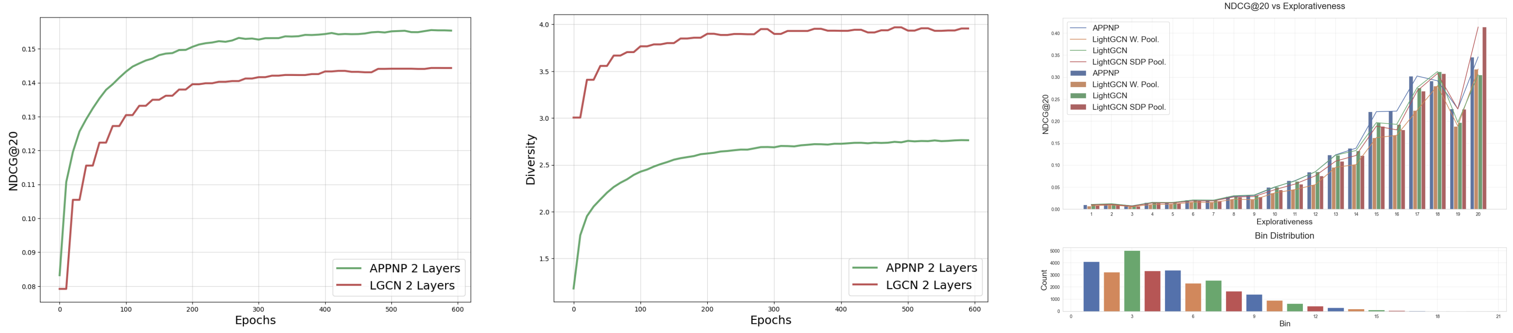
Fairness and Diversity

When comparing LightGCN and APPNP on the Gowalla dataset, APPNP comes out ahead in terms of the NDCG@20 metric, which measures the quality of recommendations. However, it doesn’t lead to more diverse recommendations. This points to the importance of looking at multiple metrics to get a full picture of a system’s performance. Additionally, it was found that both models tend to be biased towards users who have more interactions within the system, although APPNP exhibits slightly less bias. This suggests that while APPNP may give better recommendations, it still doesn’t fully solve the issue of creating a diverse set of recommendations fairly for all users.

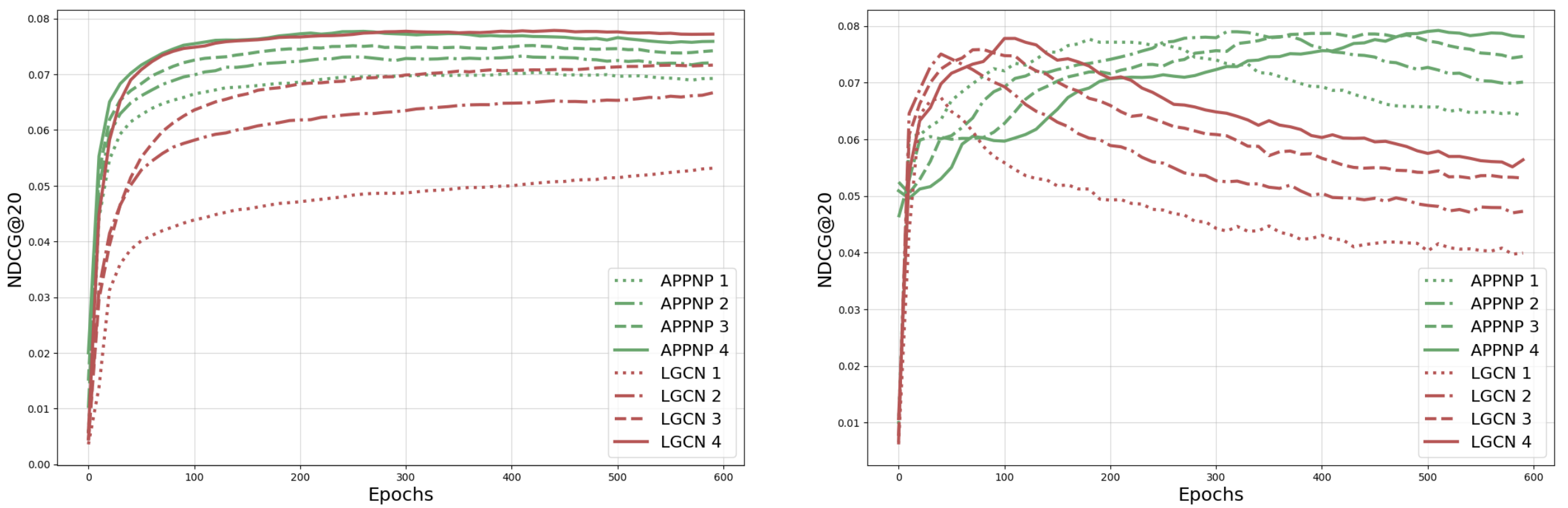
Performance

In a nutshell, adding propagation techniques to LightGCN (i.e. APPNP), stabilizes early training phases but doesn’t necessarily boost the peak performance of the recommendation system. While LightGCN sees a dip in performance partway through training on the Amazon-Electronics dataset, its counterpart, APPNP, maintains a steady performance level. This pattern holds true across various datasets tested. Essentially, while propagation aids in steadying the training journey, it doesn’t push the final effectiveness beyond what LightGCN achieves on its own.

Parting Thoughts

To sum it up, LightGCN’s performance seemed to favour users with a high number of interactions and propagating the embeddings through diffusion generally yields better results than LightGCN. Merging LightGCN with APPNP requires more extensive training and fine-tuning. Future work can consider approaches like Dual LightGCN for graded interaction predictions, integrating graph attention networks for complex relationship capture and understanding how dataset properties such as sparsity and graph size impact diffusion parameters. Check our paper to see the numbers and plots!

---

If you made it this far, I hope you enjoyed the read and learned something new! If you have any questions, feel free to reach out to me on Twitter or LinkedIn. I’d love to hear your thoughts! 😊